Variable-EDO Triads in 3D — Lissajous Curves + Overtone Playback in Desmos

Overview:
This project is a Desmos (3D) implementation by Reiji (age 9). A triad built in an arbitrary equal division of the octave (EDO 1–1200) is visualized as a 3D Lissajous curve, while the corresponding three tones are played simultaneously using Desmos tone() with an adjustable overtone range (1–128).

The goal is to observe how close an EDO triad is to simple just ratios (e.g. \(5/4\), \(3/2\)), using two linked perspectives: (1) visual cues such as how “regular” or “closed” the curve appears, and (2) auditory cues such as beating (wobbling) that can arise from mismatches between certain partials when overtones are enabled.

Notes on interpretation:
“Closer” and “farther” are not defined here as a strict numeric error metric. Instead, they are treated as observational signs, mainly: (i) the curve looks more regular / closes more cleanly, and (ii) beating becomes less prominent. Also, 2D projections (XY / XZ / YZ) can look different even for the same frequency ratios, because the appearance depends on the chosen coordinate representation (including the role/order of \(\sin\) and \(\cos\)).

Note: All content on this page is originally explained by Reiji in Japanese. The English version is translated by AI and structured by a parent, with Reiji's final approval.

Reiji's Words and Ideas

• What this is
  I built a system that draws a triad in any EDO (from 1 to 1200) as a 3D animated Lissajous curve, and plays the corresponding three tones at the same time. In 3D, relationships that can be hard to see as a “triad” in 2D projections can become clearer as a spatial structure. The sound is linked to the visualization, so I can listen to the triad while watching the curve.
• Formulas (Lissajous part)
  \[ \left(\sin At,\ \cos Bt,\ \sin Ct\right) \] This is a parametric representation used to draw the 3D Lissajous curve.
  
  \(A\): the first tone. Since this is the root, it is fixed to 1.
  \(B\): the second tone: \[ B=\sqrt[e_{do}]{2}^{s_{tep}} \] \(C\): the third tone: \[ C=\sqrt[e_{do}]{2}^{s_{tep2}} \] (I keep the expressions for \(B\) and \(C\) in the same form as in Desmos.)
• Formulas (tone playback)
  Root tone: \[ \operatorname{tone}\left(h_{z}\cdot\left[1...o_{vertone}\right]\right) \] Second tone: \[ \operatorname{tone}\left(\left(h_{z}\cdot2^{\frac{s_{tep}}{e_{do}}}\right)\cdot\left[1...o_{vertone}\right]\right) \] Third tone: \[ \operatorname{tone}\left(\left(h_{z}\cdot2^{\frac{s_{tep2}}{e_{do}}}\right)\cdot\left[1...o_{vertone}\right]\right) \] Overtones can make small mismatches easier to hear as beating between specific partials.
• Variables
  
  • overtone (\(o_{vertone}\)): sets how many overtones are played (1–128). If it is 1, it is a single sine partial.
  • u: how far forward in time to draw (0 to \(60\pi\)). This helps find points where the curve almost fully closes.
  • edo (\(e_{do}\)): sets the equal division of the octave (1–1200).
  • step (\(s_{tep}\)): which step above the root is used for the second tone.
  • step2 (\(s_{tep2}\)): which step above the root is used for the third tone.
  • h (\(h_{z}\)): the root frequency in Hz.
  If the system becomes heavy on a device, lowering overtone can help.
• Why the projections can look different
  For example, in 12-EDO with a C–E–G triad: XY shows the C–E relationship, XZ shows the C–G relationship, and YZ also relates to C–E. However, YZ does not necessarily look identical to XY.
  
  This is because in the XY plane, it is represented by the pair \(x=\sin (y)\), \(y=\cos (x)\), while in the YZ plane the roles of the axes are swapped, and the \(\sin/\cos\) assignments or ordering changes. So even when the interval content is the same, the visible features can differ depending on the chosen coordinates. I found it interesting that “the same thing” can look different depending on how it is observed.

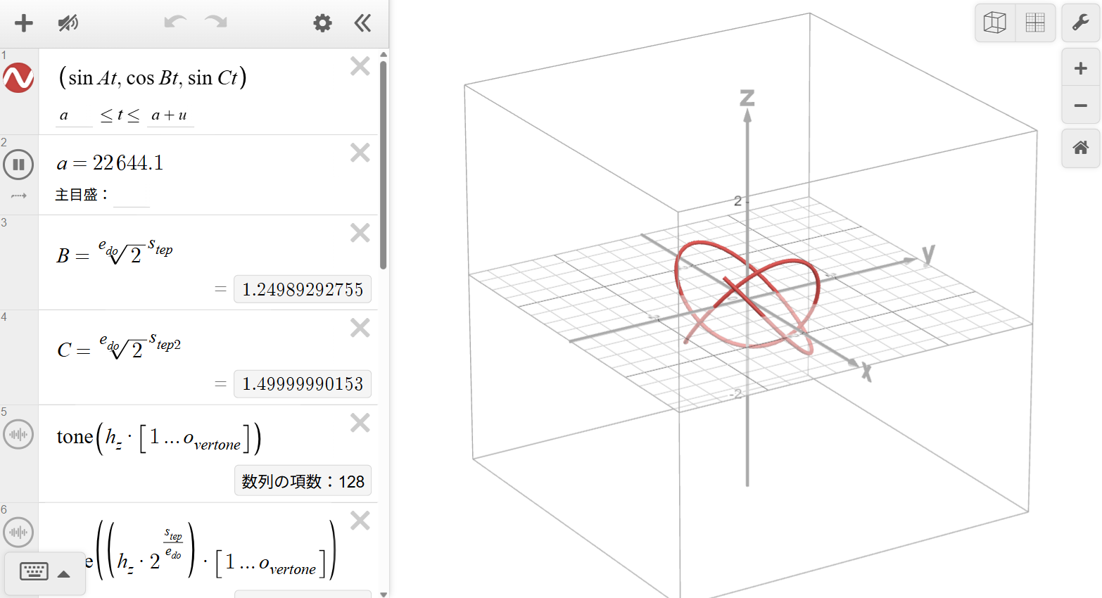
Main View: 3D Lissajous Triad with Variable EDO

A triad drawn as \((\sin At,\cos Bt,\sin Ct)\) while playing the corresponding tones using tone().
The curve’s closure and regularity are used as visual cues when comparing EDO triads to simple just ratios.

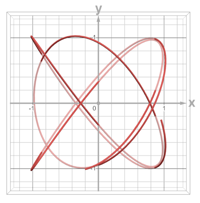
XY Projection: Root–Second Tone (A–B)

Projection onto the XY plane. When a two-tone ratio is close to a simple rational relationship, the curve often appears more regular.
With more overtones, small mismatches may become audible as beating between certain partials.

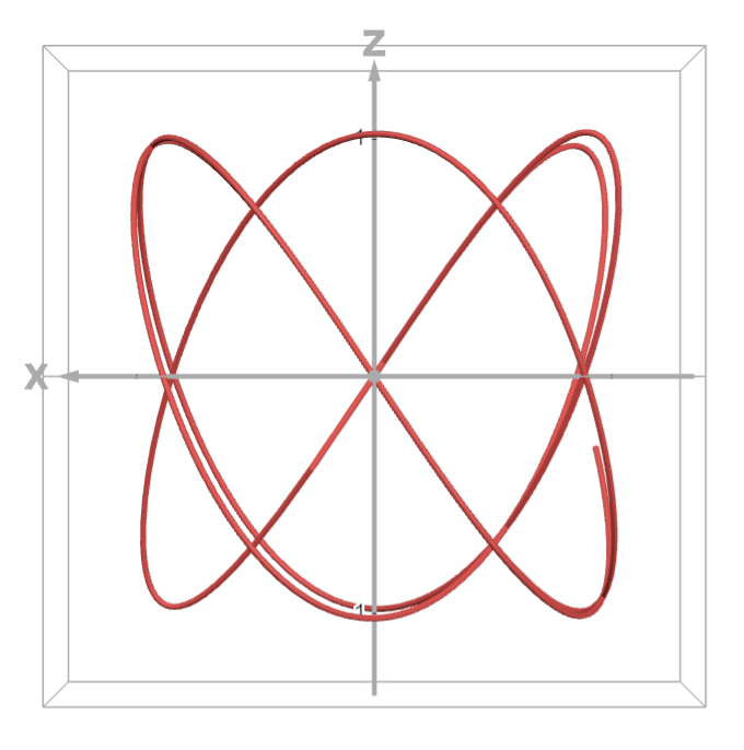
XZ Projection: Root–Third Tone (A–C)

Projection onto the XZ plane. The appearance changes with the chosen EDO and steps, reflecting how the third tone relates to the root in frequency ratio.

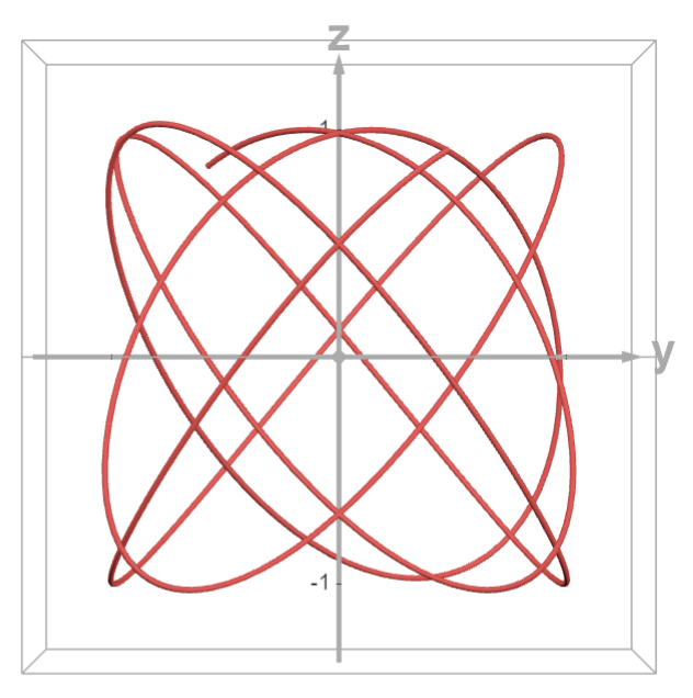
YZ Projection: Second–Third Tone (B–C)

Even when the interval content is the same, projections can look different because the coordinate roles and the \(\sin/\cos\) ordering can change across planes.

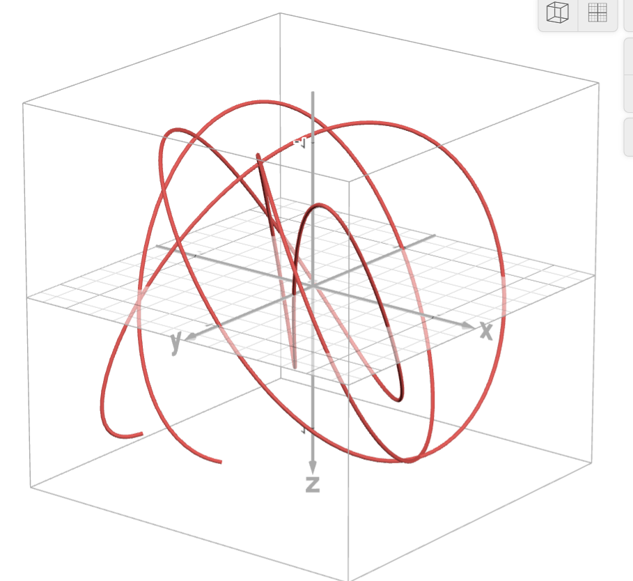
3D Shape: Observing How a Triad “Closes” in Space

The simultaneous relationship among the three tones (A, B, C) is examined as a 3D structure. A “triad” that can look overly complex in 2D can appear more simply in 3D.

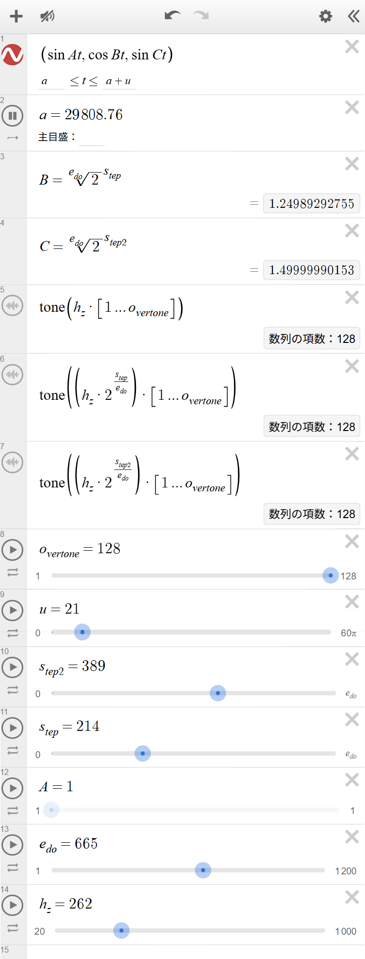
Parameter Example: EDO=665 Approximating Simple Just Ratios

Example settings \(e_{do}=665\), \(s_{tep}=214\), \(s_{tep2}=389\) yield values like \(B\approx1.2498929\) and \(C\approx1.4999999\) in Desmos, close to ratios such as \(5/4\) and \(3/2\).